NEURAL RADIANCE FIELDS
Quang Nguyen, SID: 3036566521
Project Overview
In this project, I implemented two simplified version of Neural Radiance Field that can fit a 2D Image and Multi-view Images respectively.
PART 1: FIT A NEURAL FIELD TO 2D IMAGE
1.1. Network
My model has a similar architecture to the one referenced on the project spec. Each coordinate (x,y) is passed into a positional encoding layer, which converted a B x 2 input tensor to an encoded B x 4L+2 output tensor. This layer is followed by a Multilayer Perceptron (MLP) network with three hidden linear layers of dimension 256 and a final linear layer of size 3. Each hidden linear layer is followed by a nn.ReLU while the final output layer is followed by a nn.Sigmoid.
1.2. Dataloader
Rather than implementing a random sampling dataloader with torch.Dataset, which takes an absurd amount of time to run for a small image, I directly sample new N pixels for every training iteration. This allows the model to run much faster and more efficiently.
1.3. Hyperparameter Tuning for Fox
1.3.1. Learning Rate
The first parameter that I tuned is the learning rate, which I varied by a factor of 10. We can see that The best learning rate that 0.01 and 0.001 yield similar performance while 0.0001 is slight worse. 1e-05 wasn't able to converge in 5000 iterations because it is too low, suggesting that if trained for longer, this learning rate might still be to achieve a similar PSNR with the other learning rates. Both 0.1 and 1 are too high and they both converge to an extremely high value of training loss and low value of training PSNR. In the end, I decided on using lr=0.001, the green curve in the graph that seems to converge to the highest PSNR value.
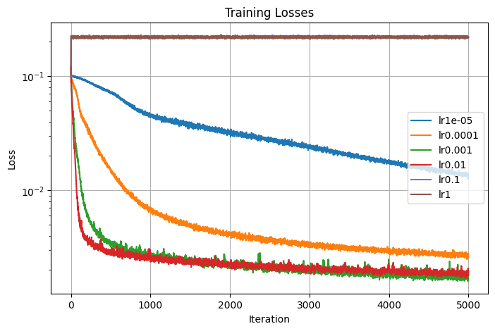
Losses
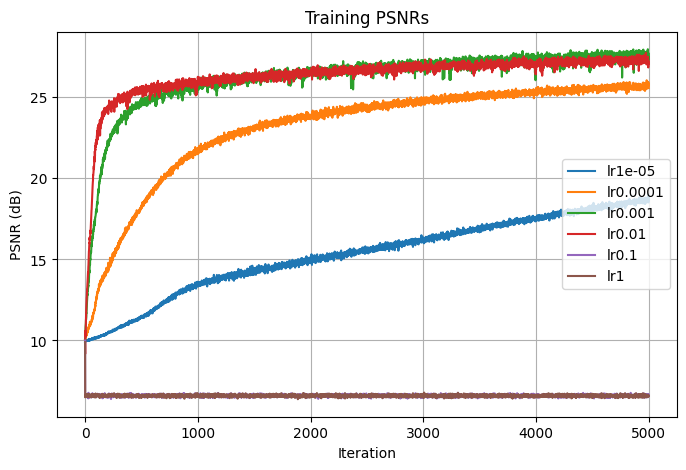
PSNRs
1.3.2. Highest Frequency Level of the Positional Encoding layer
The next parameter that I tuned is the highest frequency level of the positional encoding layer, which I varied by 5. When the frequency level is 5, the model performs the worse both in terms of PSNR and loss. For higher frequency levels between 10 and 25, they yield similar performance in PSNR. In the end, I decided on using L=20, the red curve in the graph that seems to converge to the highest PSNR value.
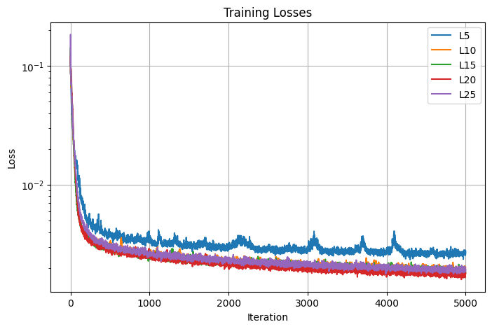
Losses
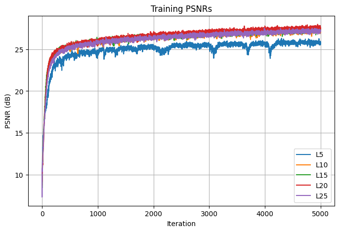
PSNRs
1.4. Final Result for Fox
The final result for the fox image was generated using the model architecture as descrived above, a learning rate of 0.001, and L=20. This model is then trained over 5000 iterations. Here are the output images obtained every 100 iterations in the first 1000 iterations:

Iter 0
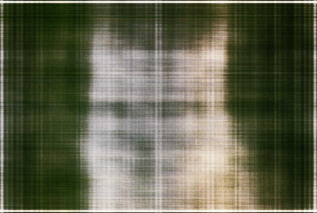
Iter 100
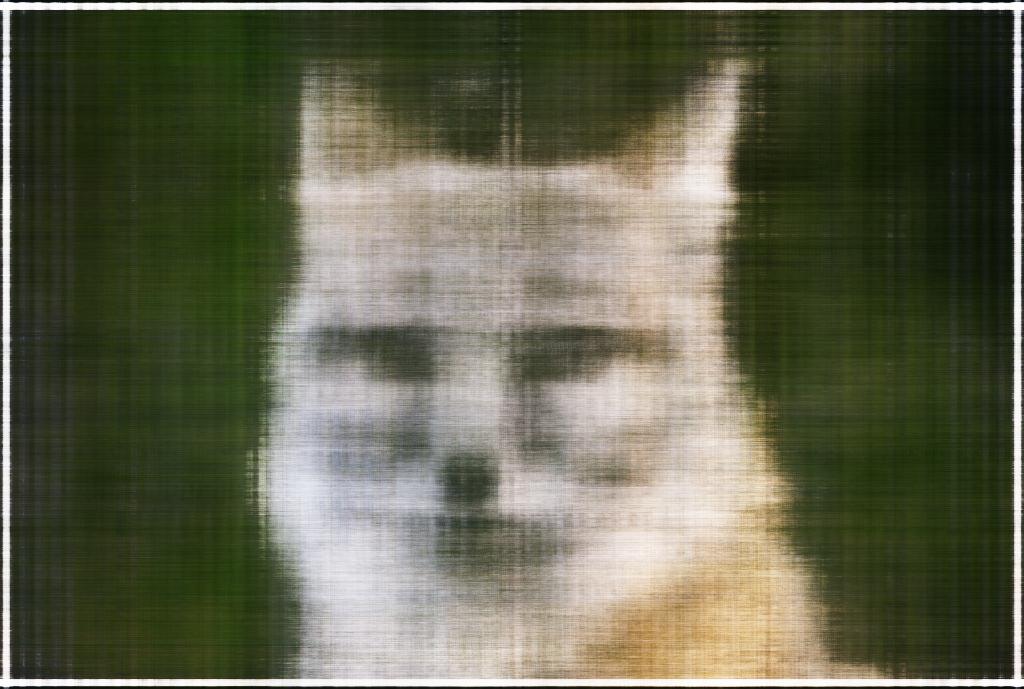
Iter 200

Iter 300
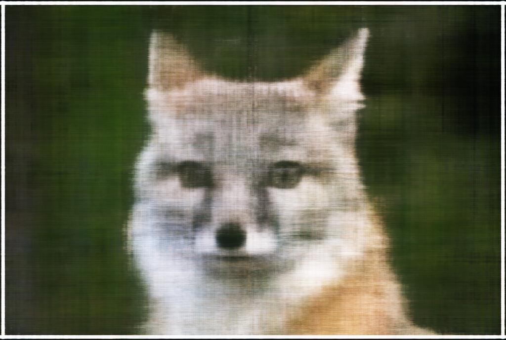
Iter 400
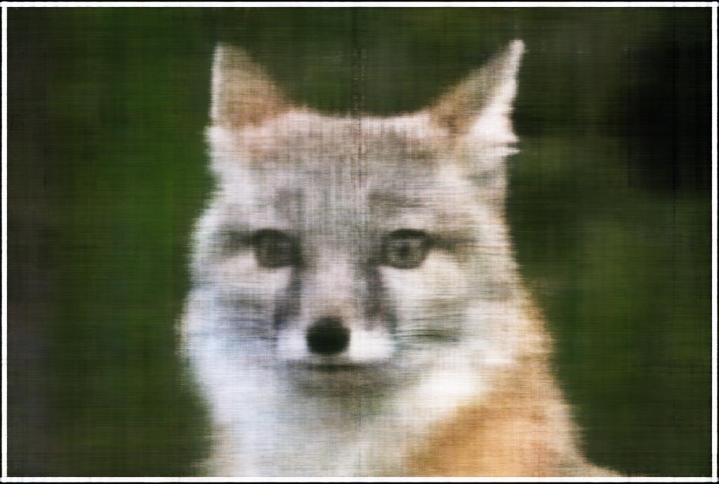
Iter 500

Iter 600
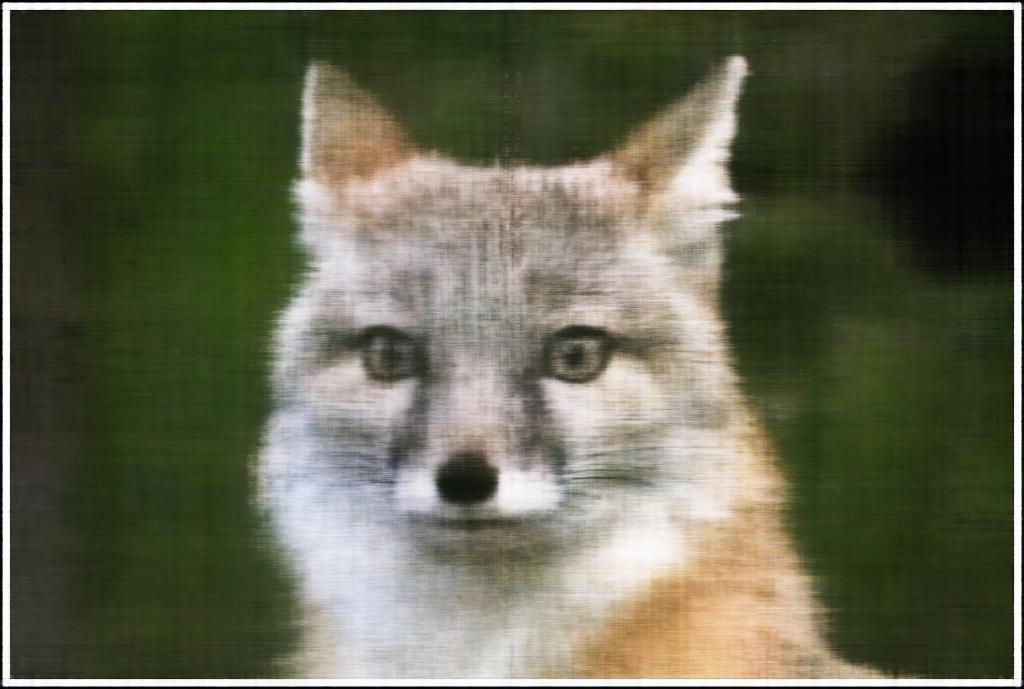
Iter 700
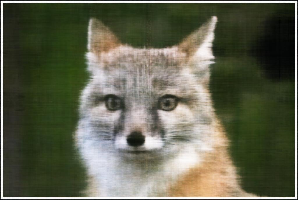
Iter 800

Iter 900

Iter 1000
Here are the training losses and psnrs curve for the final result:
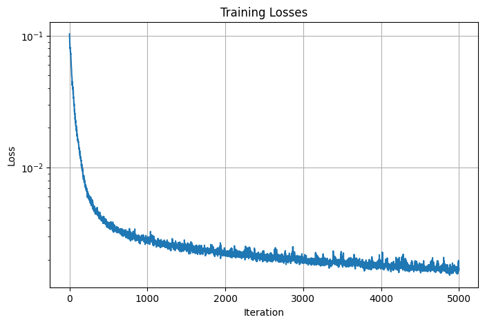
Losses
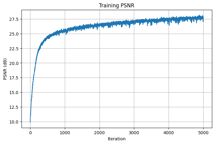
PSNRs
Here is the final result in comparison with the input image:
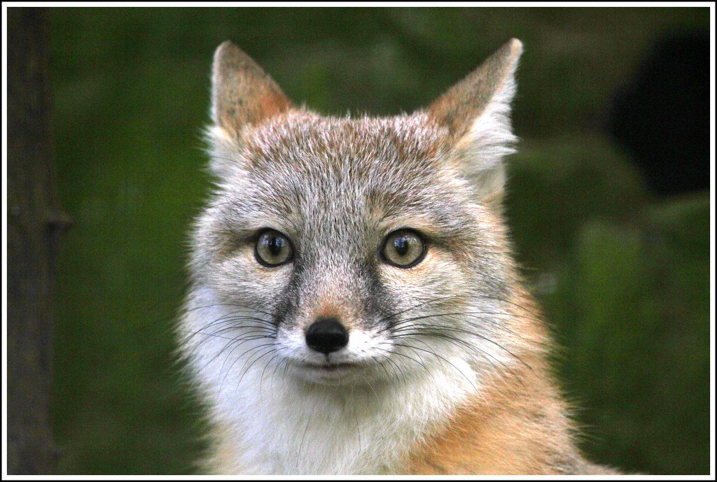
Input Image
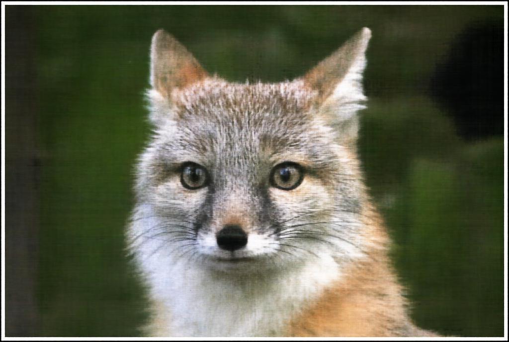
Final reconstructed fox with PSNR=27.85
1.5. Hyperparameter Tuning for Notre Dame
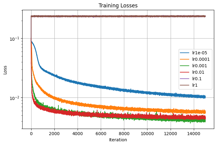
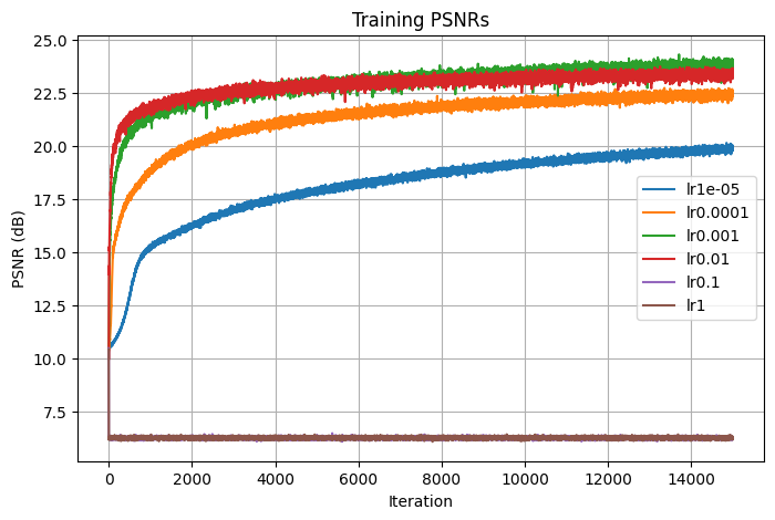
1.5.1. Learning Rate
The first parameter that I tuned is the learning rate, which I varied by a factor of 10. I decided on using the best learning rate lr=0.001, the green curve in the graph that seems to converge to the highest PSNR value.
Losses
PSNRs
1.5.2. Highest Frequency Level of the Positional Encoding layer
The next parameter that I tuned is the highest frequency level of the positional encoding layer, which I varied by 5. I decided on using the best max frequency L=10, the orange curve in the graph that seems to converge to the highest PSNR value.
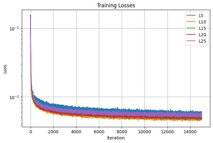
Losses
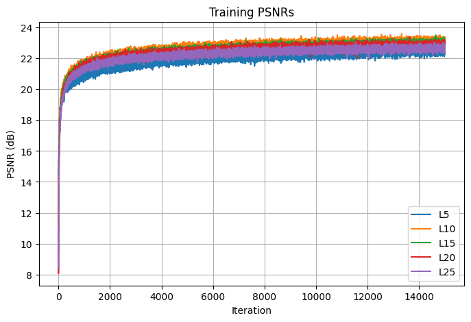
PSNRs
1.6. Final Result for Notre Dame
The final result for the Notre Dame image was generated using the model architecture as descrived above, a learning rate of 0.001, and L=10. This model is then trained over 15000 iterations. Here are the output images obtained every 100 iterations in the first 1000 iterations:

Iter 0
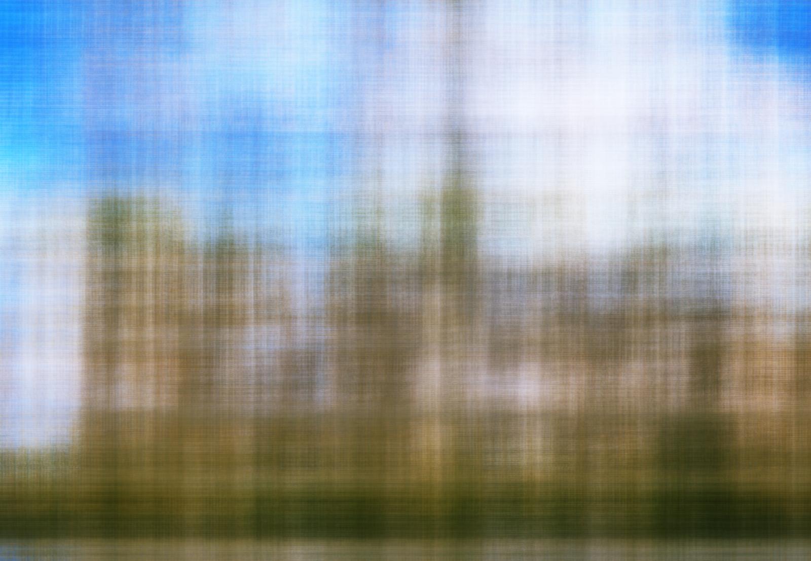
Iter 100
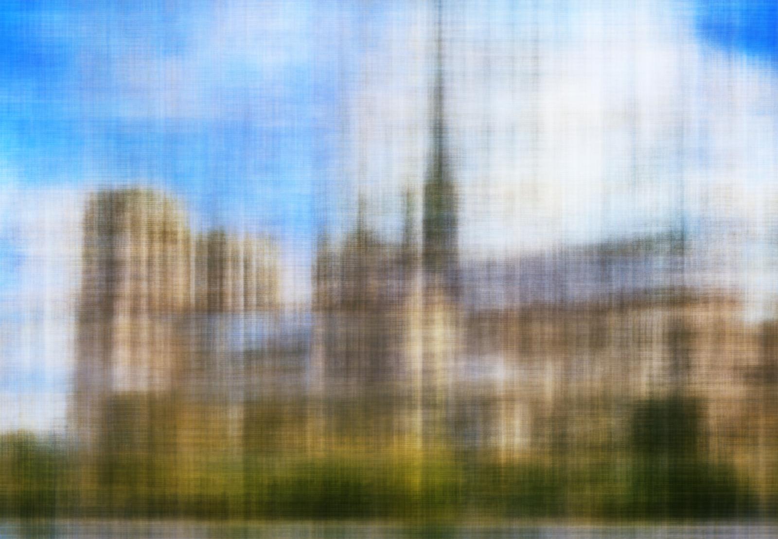
Iter 200
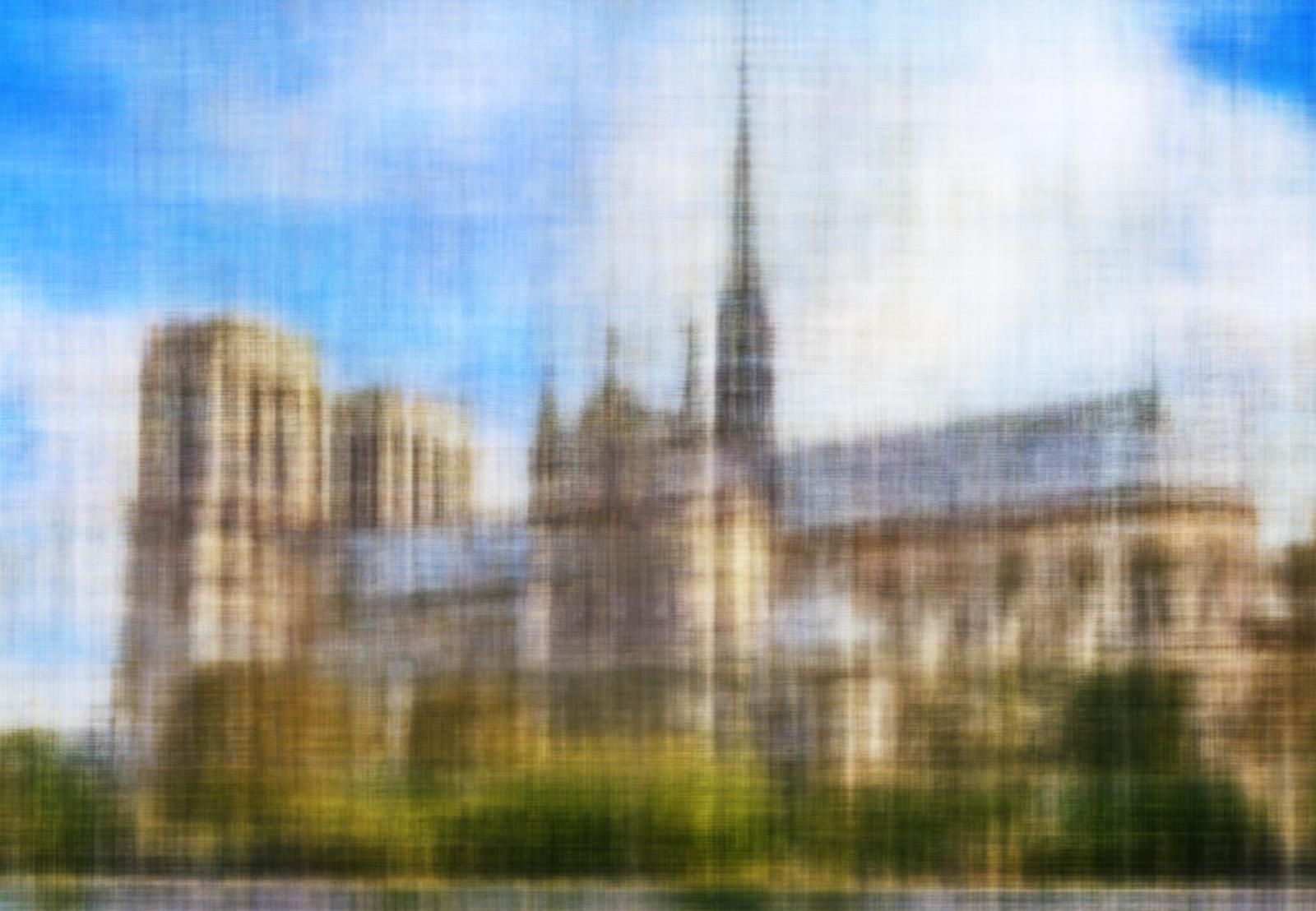
Iter 300

Iter 400
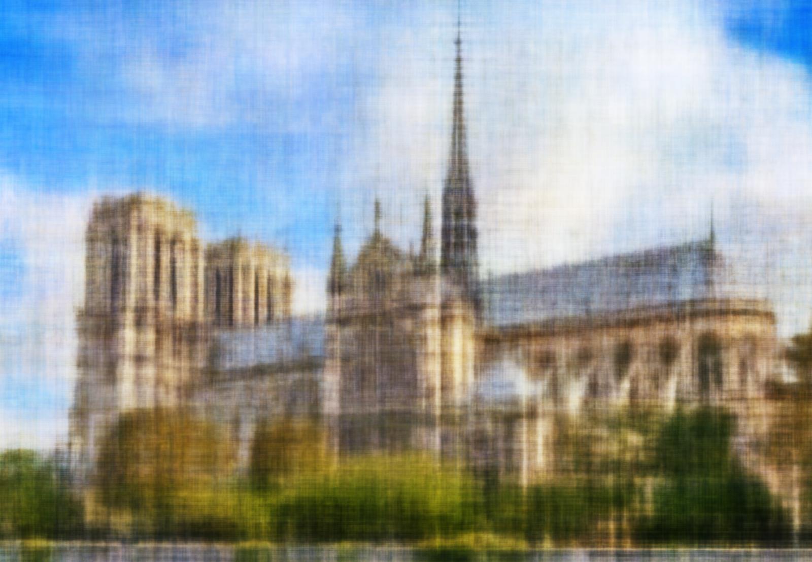
Iter 500
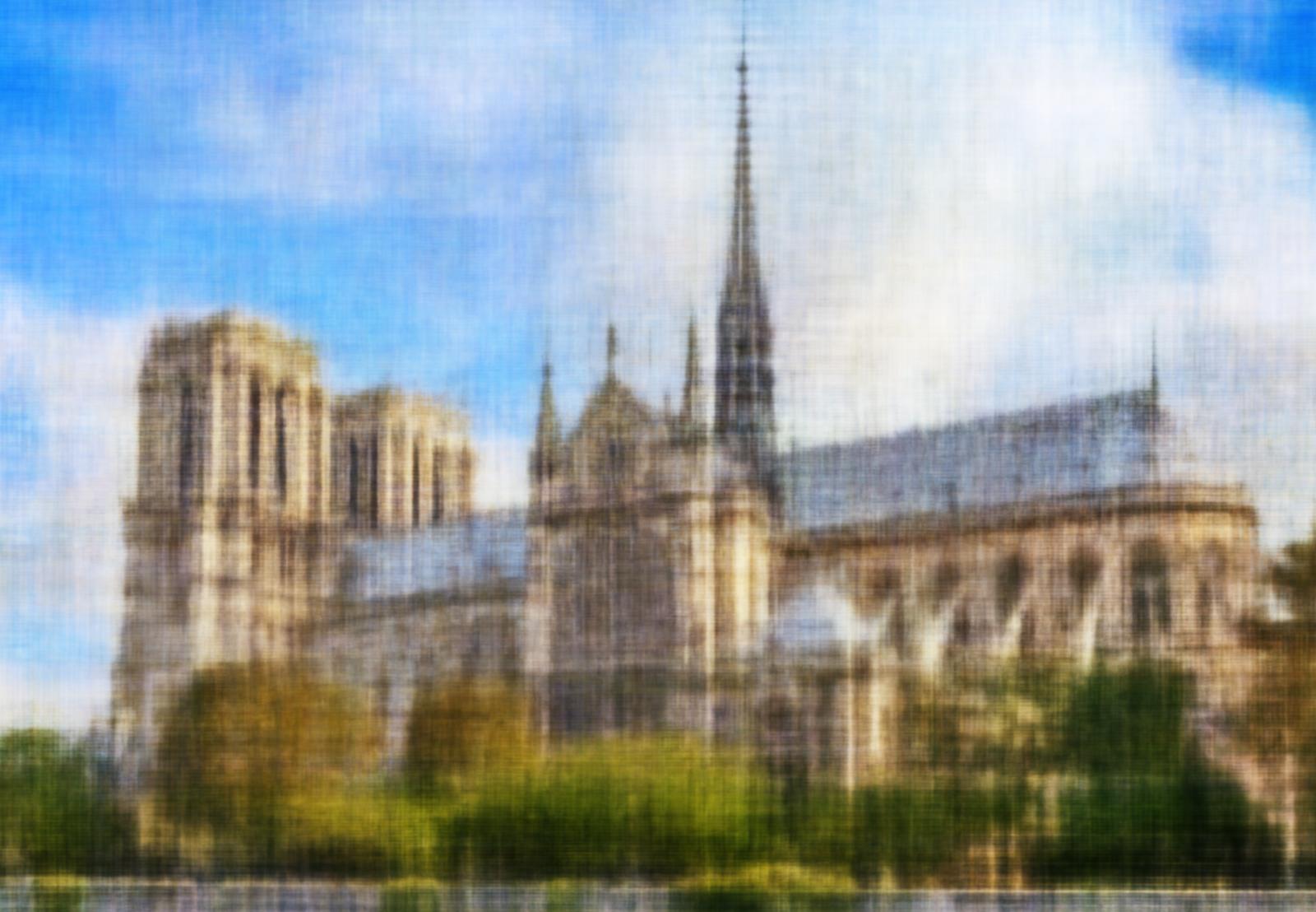
Iter 600
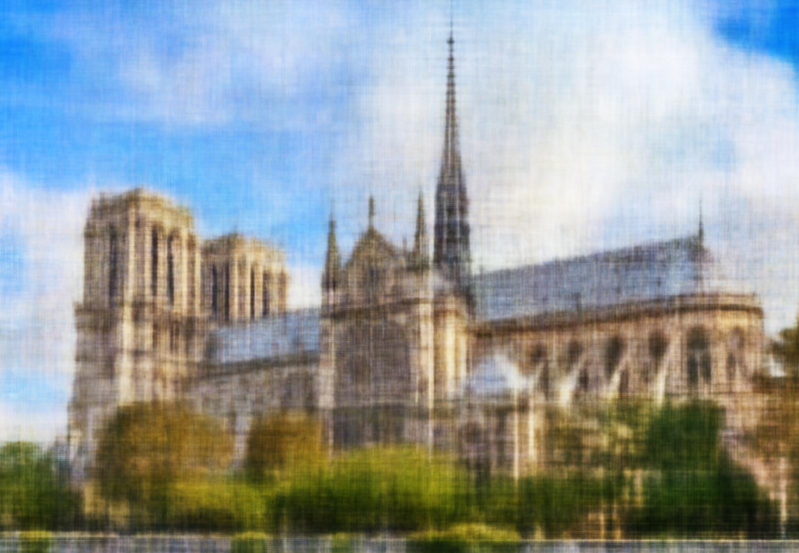
Iter 700
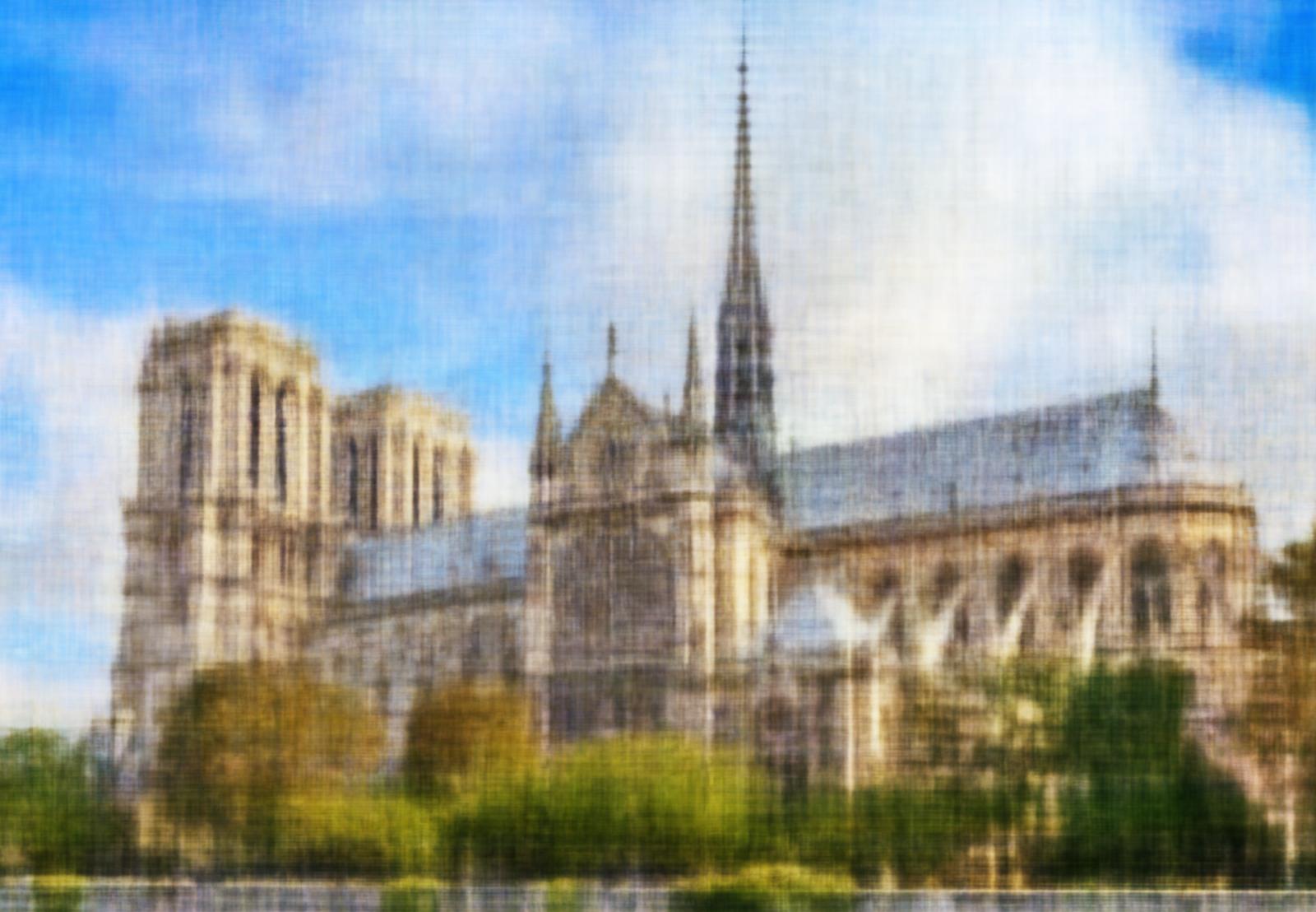
Iter 800

Iter 900
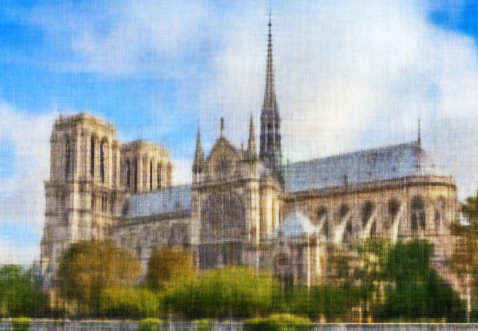
Iter 1000
Here are the training losses and psnrs curve for the final result:
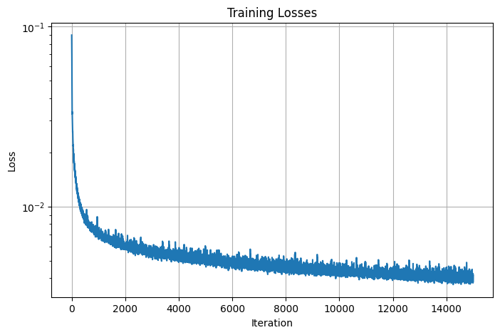
Losses
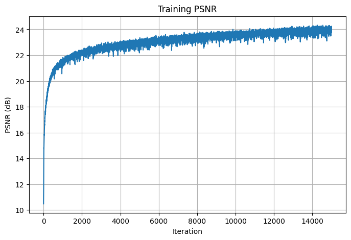
PSNRs
Here is the final result in comparison with the input image:
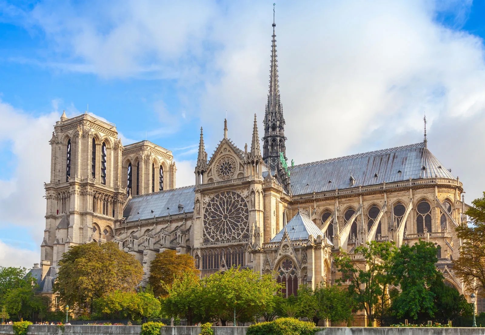
Input Image

Final reconstructed Notre Dame with PSNR=24.01
PART 2: FIT A NEURAL FIELD TO FROM MULTI-VIEW IMAGES
2.1. Create Rays from Cameras
2.1.1. Camera to Wolrd Coordinate Conversion
To implement transform(c2w, x_c), I first concatenated ones to the batched 3D coordinates x_c to obtain the batched 3D homogenous coordinates x_c_ones. I then transposed them such that their dimension is consistent with the equation setup and used torch.bmm to right multiply c2w with the transposed coordinates. Finally, I returned the resulting world-space coordinate by indexing the output of the matrix multiplication and ignore all the ones.
2.1.2. Pixel to Camera Coordinate Conversion
To implement pixel_to_camera(K, uv, s), I first concatenated ones to the batched 2D coordinates uv to obtain the batched 2D homogenous coordinates uv_ones. I then reshaped uv_ones to swap the x- and y- coordinates accordingly and used torch.bmm to right multiply K.inverse() with the reshaped uv_ones. Finally, I transposed the output of this multiplication such that its dimension and view is consistent with the rest of the project and return its product with s, which gives the transformed coordinates in camera space.
Note that K, the intrinsic matrix, is constructed with o_x=image_width/2, o_y=image_height/2, f_x=f_y=focal where focal=data["focal"] given by the input file.
2.1.3. Pixel to Ray
To implement pixel_to_ray(K, c2w, uv), I first obtained the camera-space coordinates with x_c = pixel_to_camera(K, uv, s) where s is just a tensor of ones. Then, I extracted R, t by indexing properly from w2c = torch.inverse(c2w) and computed ray_o by right multiply -R.inverse with t using torch.bmm. To acquire ray_d, I first obtained the world-space coordinates by calling transform(c2w, x_c) and subtracted ray_o from this result. Finally, I returned ray_o and the normalized version of ray_d.
2.2. Sampling
2.2.1. Sampling Rays from Images
The function sample_rays(batch_size, single=False, single_idx=None) is implemented as followed: I first flattened pixels and rays from all images with reshape(-1,3). single is to denote whether I wanted to retrieve batch_size rays from all images or whether I want to retrieve all the rays of a desired image with index single_idx. If single=False, then I acquired batch_size random indices with torch.randint(0, pixels.shape[0], (batch_size,)) and returned the appropriately indexed rays and pixels. This is the random sampling that will be used in training and validation.
If single=True, then single_idx is not None and will represent the camera/image index whose rays we want to obtain. This was used during volume rendering, where I inputted the camera index of the camera test set to obtain the desired rays for reconstruction.
2.2.2. Sampling Points along Rays
To implement sample_along_rays(ray_o, ray_d, near=2.0, far=6.0, num_samples=64, pertubation=True), I first computed t = torch.linspace(near, far, num_samples, device=ray_o.device) and t_width = (far-near)/num_samples. If pertubation=True, then I will small random noise torch.rand(t.shape, device=t.device) * t_width to t so that every location along the ray would be touched upon. Finally, I returned the obtained 3D coordinates from adding ray_o + ray_d * t.
Note that I used the default parameters for this function: near=2.0, far=6.0, and num_samples=64.
2.3. Putting the Dataloading all Together
For Dataloading, I implemented the class RaysData(images, K, c2ws). It is initialized with images, the intrinsic matrix K, and the corresponding c2w cameras. The uvs used in sample_rays will also be initialized here. rays_o, rays_d are also defined as this class's instance variable through pixel_to_ray(self.Ks, self.c2ws, self.uvs) to simplify sampling rays from images. This class will have two functions: __init__ and sample_rays, which is the function described above.
uvs is intialized as followed: three torch tensors ns, ys, xs will be defined where ns=torch.arange(num_images), ys=torch.arange(image_height), and xs=torch.arange(image_width). That is, to obtain the ground truth pixel value at coordinate (x,y), in image n, we query self.images[n, y, x]. I then stacked these three tensors with torch.tensor to obtain self.uvs. Finally, I added 0.5 to the xs and ys in self.uvs to account for the offset from image coordinate to pixel center.
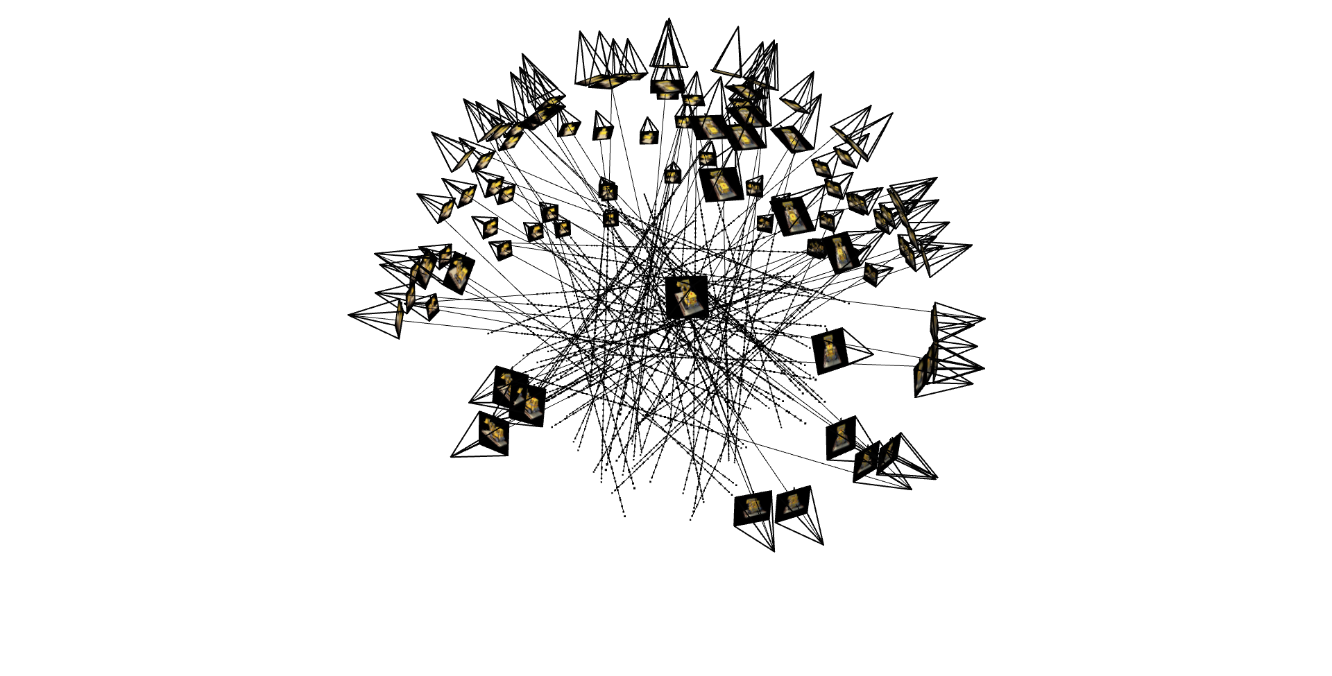
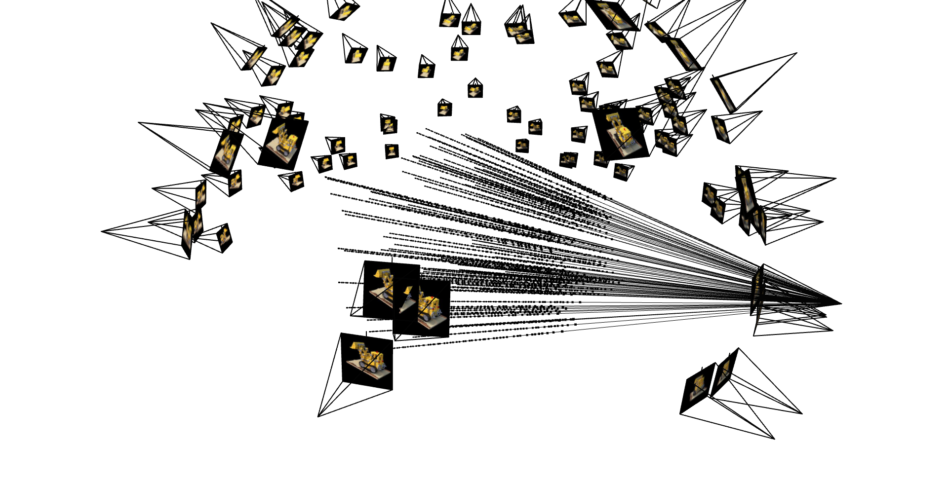
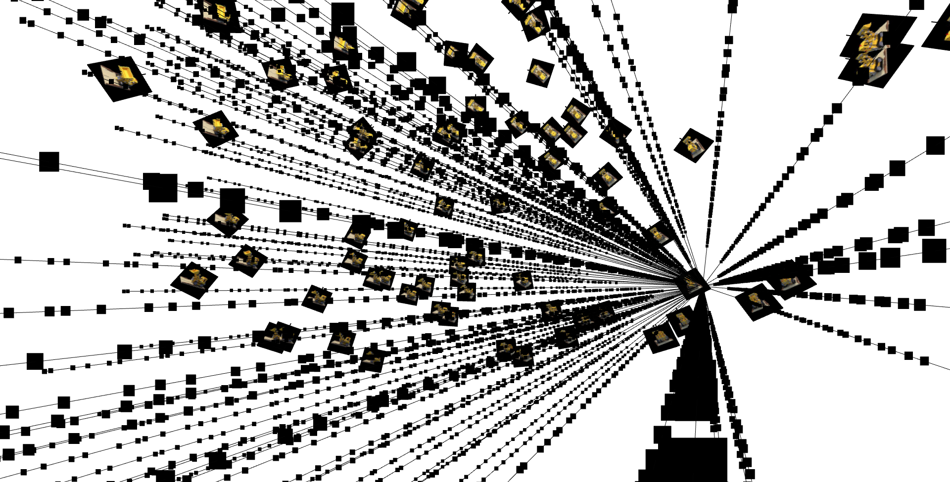
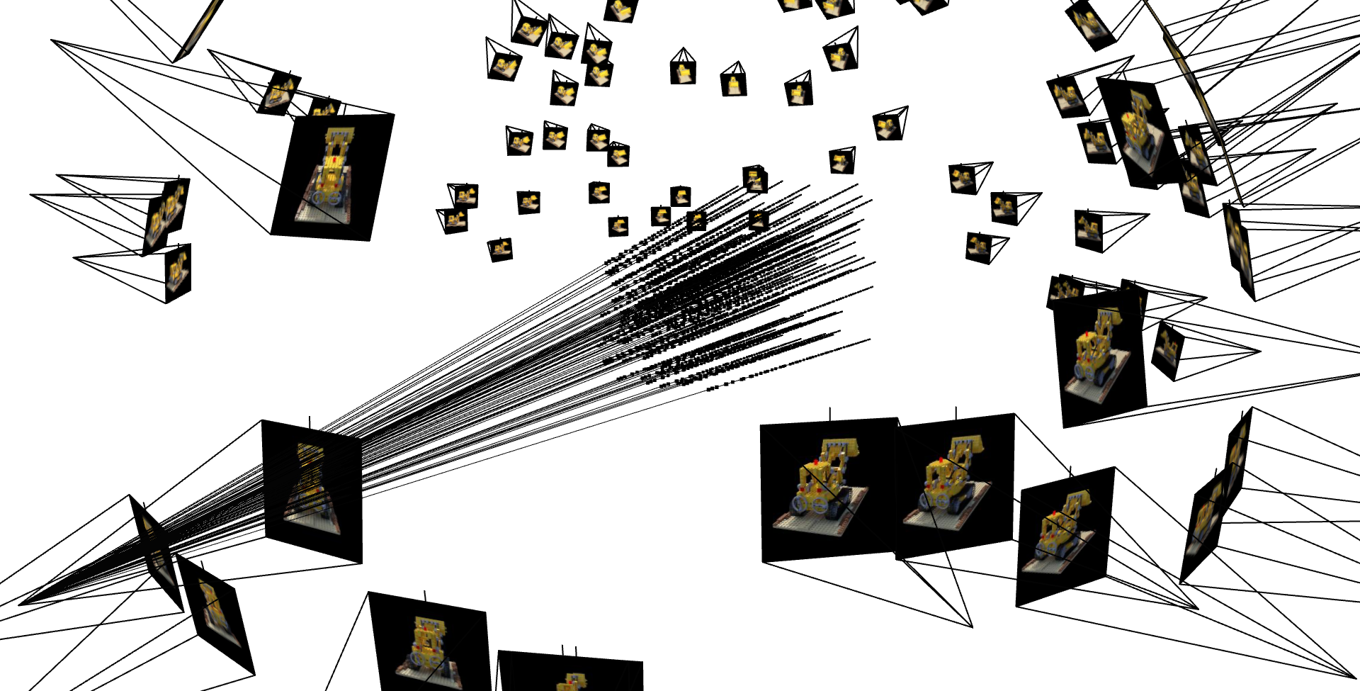
Here are the visualizations of rays and samples that I obtained using the implemented functions and RaysData:
2.4. Neural Radiance Field
I used the same model architecture as project website. I then split the network into 5 smaller subnets at each of the concatenation and implemeted them using nn.Sequential. I used default hyperparameters for my implementation; that is, L_x=10, L_ray_d=4, and hidden_dim=256.
2.5. Volume Rendering
To implement volrend(sigmas, rgbs, step_size), I first obtained prod=sigmas * step_size and computed the T_i's with torch.exp(-step_size * torch.cumsum(sigmas, dim=1) + prod). I needed to subtract (addition after distributing the negative sign) prod from the cumulative sum because exponent of the T_i is the sum of the sigma-delta products up to but excluding i. I then returned the rendered colors torch.sum(Ts * (1 - torch.exp(-prod)) * rgbs, dim=1).
2.6. Final Result
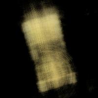
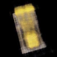
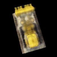
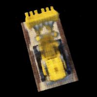
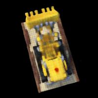
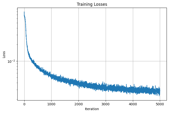
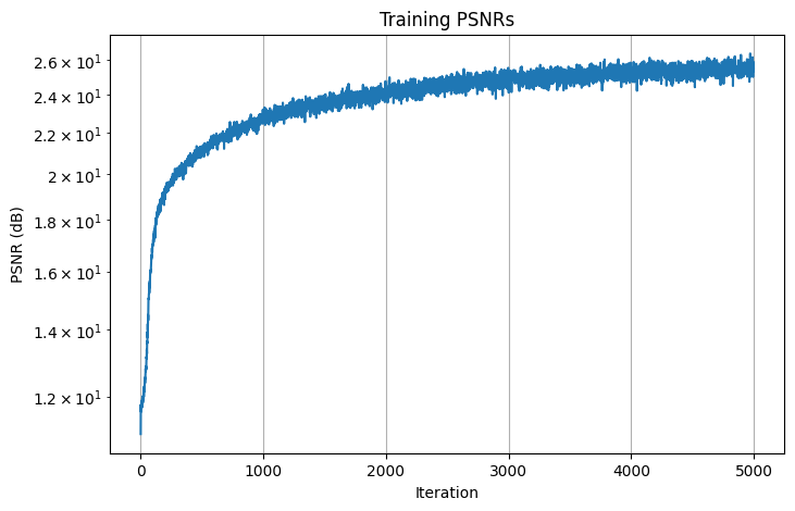
The final result for the input was generated using the model architecture as descrived above, a learning rate of 5e-4, L_x=10, L_d=4, and batch_size=10000. This model is then trained over 5000 iterations, achieving a training loss of 0.002841, training PSNR of 25.47 dB, validation loss of 0.002137, and validition PSNR of 26.70 dB. Here are the images of camera 0 from the validation set obtained at iterations 0, 100, 200, 500, 1000, 2000:

Iter 0
Iter 100
Iter 200
Iter 500
Iter 1000
Iter 2000
Here are the losses and PSNRs curve for the final result:
Training Losses
Training PSNRs
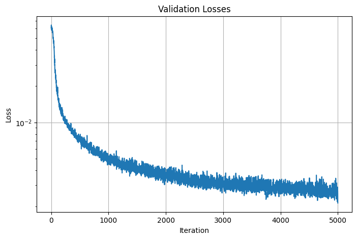
Validation Losses
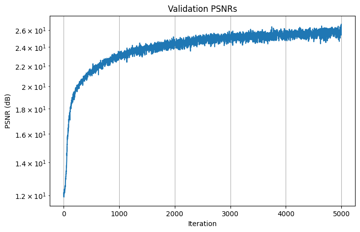
Validation PSNRs
Here is the model's predicted of rendering using the cameras from the test set:
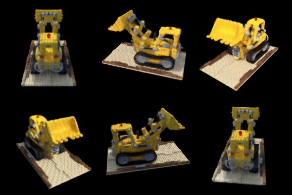
Final Rendering using the cameras from the test set
PART 3: BELL AND WHISTLES
3.1. Rendering with different background colors
To change the background color of the rendering, I modified the volrend function to take in a background color, which is a 1 x 3 RGB tensor of the desired color. I then compute the weight for the background color with background_weights = torch.exp(-torch.sum(prod, dim=1)) where prod = sigmas * step_size. Finally, I added this to the original output of the volrend function. That is, volrend_background returns torch.sum(Ts * (1 - torch.exp(-prod)) * rgbs, dim=1) + background_weights*background_color. Here is the original rendering and the rendering with a different background color side by side for comparison:

Normal Rendering
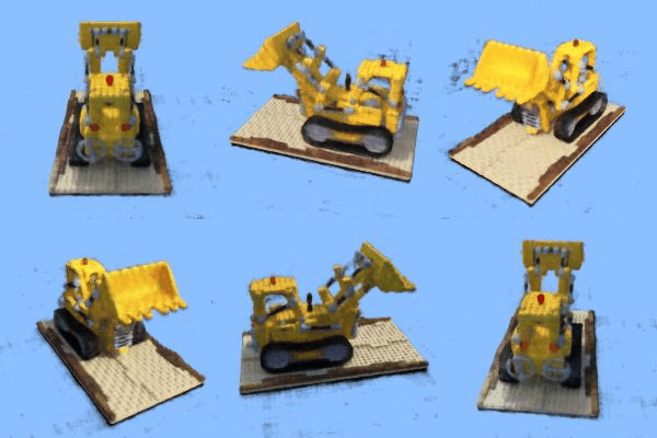
Rendering with a different background color
3.2. Rendering of depths map
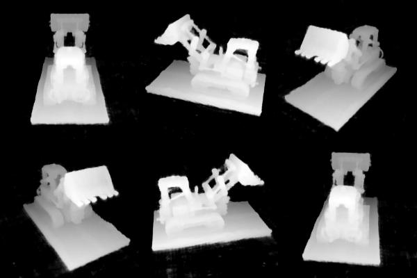
To render a depths map, I passed torch.linspace(1, 0, 64, device=pred_sigmas.device) instead of the pred_rgbs (the output of the model) into volrend when sampling. Still using the same output densities from the model, this allows the volrend function to output a depths map where darker colors denote positions farther away from the camera and light colors illustrate positions closer to the camera. Here is the original rendering and the rendering of the depths map side by side for comparison:

Normal Rendering
Rendering of depths map