FACE MORPHING
Quang Nguyen, SID: 3036566521
1. Project Overview
This project aims to build intuitions behind image warping and morphing. More specifically, I
- Produced a "morph" animation of my face into the face of George Clooney.
- Computed the mean of a population of faces from the Danes dataset.
- Extrapolated from the population mean to create a caricature of myself.
- Performed gender swap from male to female for my face.
- Used PCA basis for morphing and extrapolating.
2. Defining Correspoondences
Here are the two input portraits: one is of me and the other is of George Clooney.
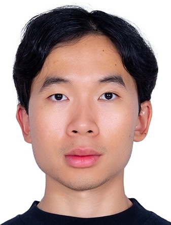
Portrait of Quang Nguyen
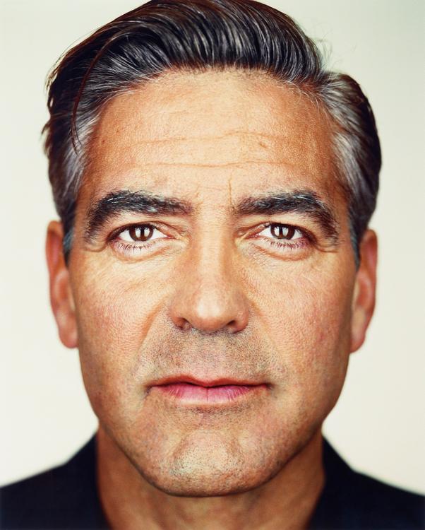
Portrait of George Clooney
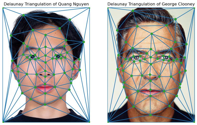
Using this labeling tool, I defined 61 keypoints (including the 4 keypoints for the 4 corners), where each of them is a pair of corresonding points on the two images. These keypoints are defined using the same ordering for the two faces. Here are the Delaunay triangulations on the point sets:
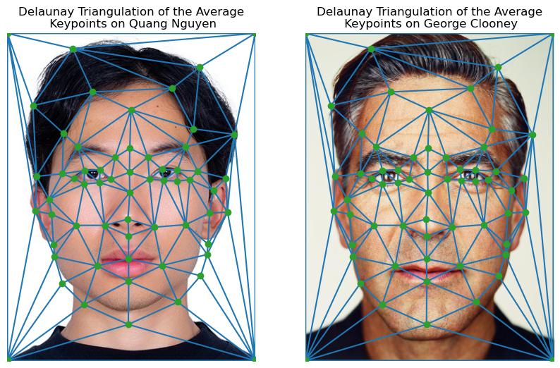
I then computed the element-wise mean of these point sets to obtain the midway shape. Here is the Delaunay triangulation of the midway shape on the two input images:
3. Computing the "Mid-Way Face"
From lecture, we define an affine transformation as follow: \[A\begin{bmatrix} x \\ y \\ 1 \end{bmatrix} = \begin{bmatrix} a & b & c\\ d & e & f\\ 0 & 0 & 1 \end{bmatrix}\begin{bmatrix} x \\ y \\ 1 \end{bmatrix} = \begin{bmatrix} x' \\ y' \\ 1 \end{bmatrix}\]
Let tri1_pts and tri2_pts be the triangle points such that \(\text{tr1_pts}=\begin{bmatrix} x_1 & y_1 \\ x_2 & y_2 \\ x_3 & y_3 \end{bmatrix}\) and \(\text{tr2_pts}=\begin{bmatrix} a_1 & b_1 \\ a_2 & b_2 \\ a_3 & b_3 \end{bmatrix}\). Then, we can express the transformation as \[A\begin{bmatrix} x_1 & x_2 & x_3\\ y_1 & y_2 & y_3 \\ 1 & 1 & 1 \end{bmatrix} = \begin{bmatrix} a_1 & a_2 & a_3\\ b_1 & b_2 & b_3 \\ 1 & 1 & 1 \end{bmatrix},\]
where \(\begin{bmatrix}
x_1 & x_2 & x_3\\ y_1 & y_2 & y_3 \\ 1 & 1 & 1
\end{bmatrix} = \)np.vstack((tri1_pts.T, np.ones((1, 3)))) and \(\begin{bmatrix}
a_1 & a_2 & a_3\\ b_1 & b_2 & b_3 \\ 1 & 1 & 1
\end{bmatrix} = \)np.vstack((tri2_pts.T, np.ones((1, 3)))). As a result, we can obtain the affine transformation matrix by doing A = tri2_pts.dot(np.linalg.inv(tri1_pts)).
With this matrix, I proceeded to compute the mid-way face by following this process:
- Compute the average shape by taking the element-wise average of the set of keypoints of the two images.
- Warp both faces into that shape by computing the affine transformation matrix of each pair of triangle and warp the triangles using those matrices. For this step, I iterated over all triangles of the average shape and for each triangle, I iterated over all the possible pixels contained in that triangle using
skimage.draw.polygonand interpolated the pixel value using a linear interpolation fromscipy.interpolate.RegularGridInterpolator. - Average the colors of the two resulting images to obtain the final mid-war face
Here is the portrait of me, the mid-way face of me, Quang Nguyen, and George Clooney, and the portrait of George Clooney:

Portrait of Quang Nguyen
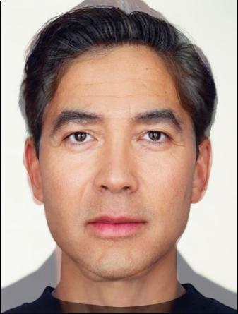
"Mid-Way" Face between Quang Nguyen and George Clooney

Portrait of George Clooney
4. The Morph Sequence
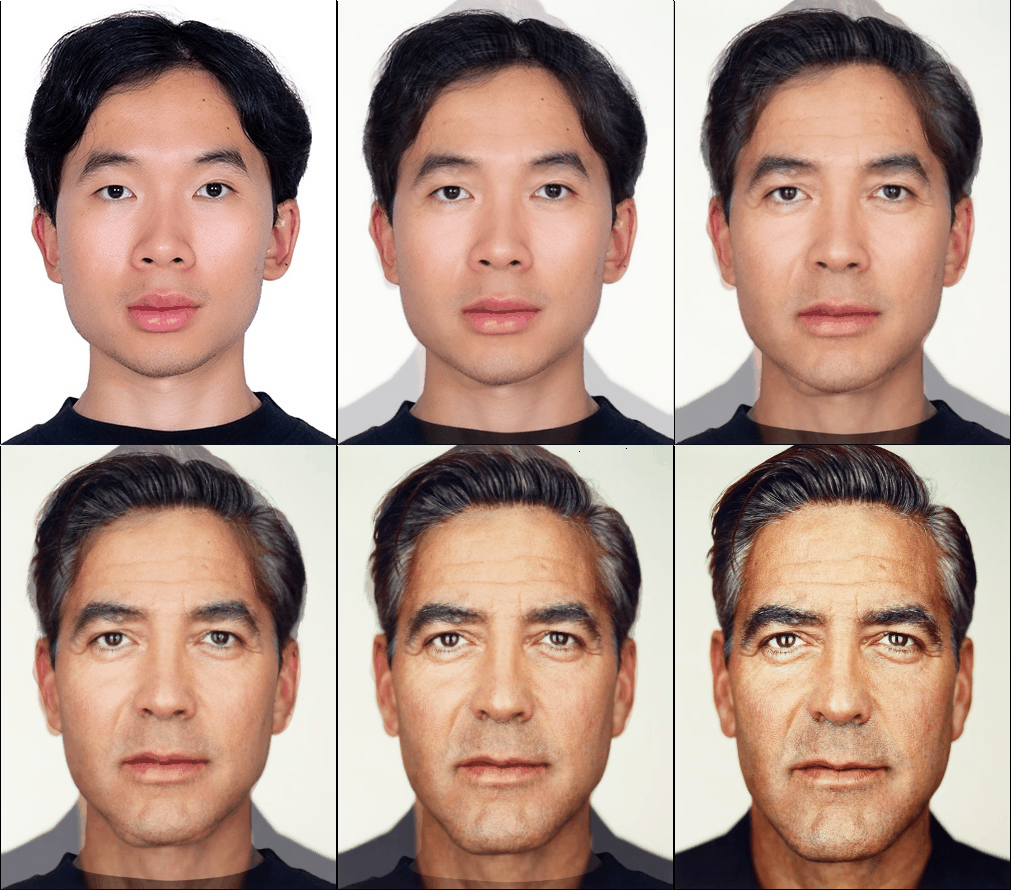
Rather than using a constant ratio \(\frac{1}{2}\) for both warping and color dissolving, I generalized the previous part into the function morph(im1, im2, im1_pts, im2_pts, tri, warp_frac, dissolve_frac) that produces a warp between im1 and im2 using warp_frac, dissolve_frac for shape warping and color dissolving, respectively. By jointly ranging the two fractions together from 0 to 1 with a total of 45 frames through the use of np.linspace(0, 1, 45), I generated video sequence of a morph from my portrait to the image of George Clooney. Here's the gif of that video sequence:
5. The "Mean Face" of a Population
I used the initially released subset of the IMM Face Database (i.e. the Danes dataset). For this part, I used the entire population (37 images) rather than singling out a subpopulation.
Here is a different portrait of me that better aligns with a Dane image and contains the appropriate keypoints (similar number and in the same order) as the annotations for the Danes dataset:
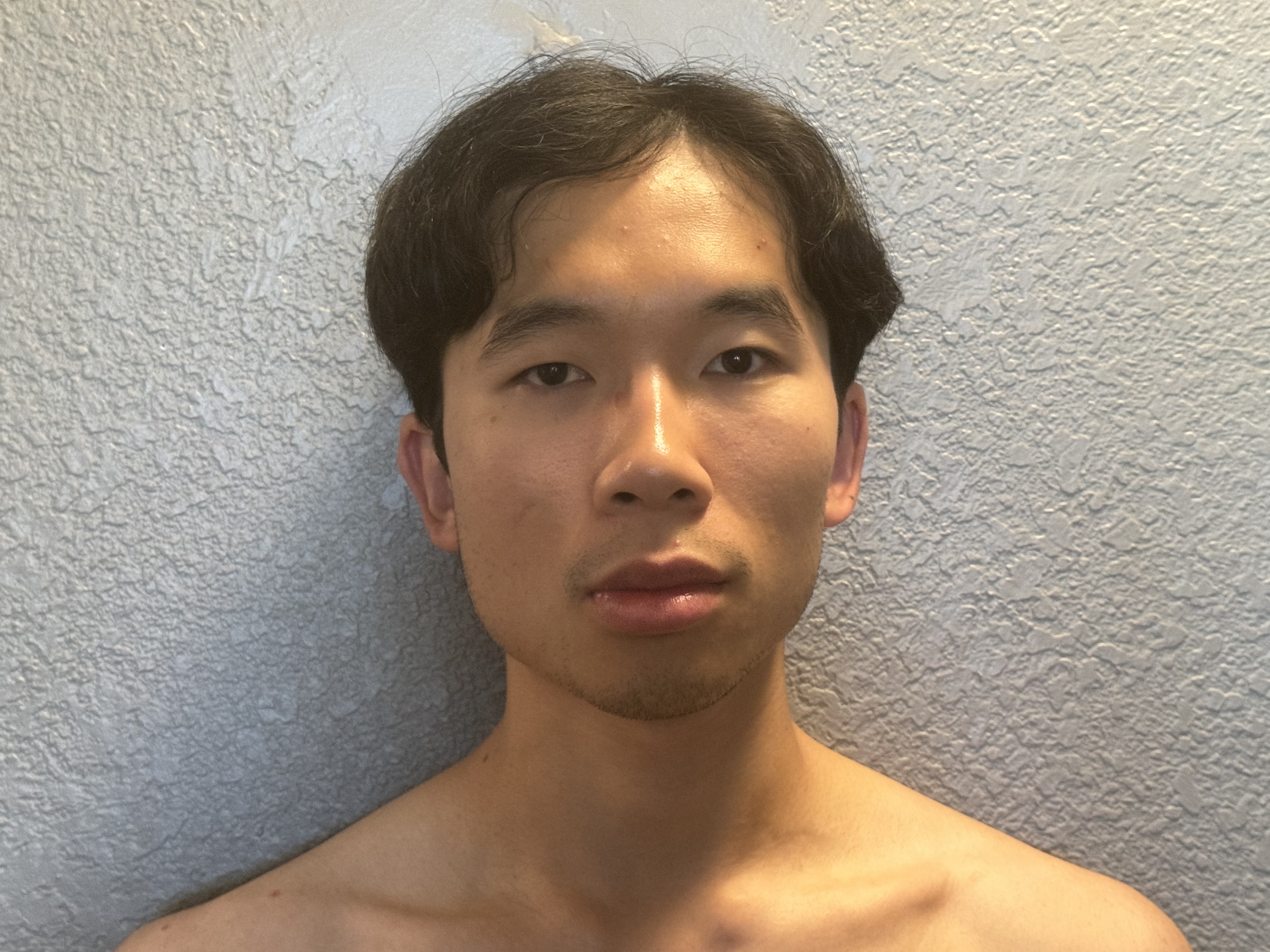
I extracted the keypoints for each Dane from the .asf file and for each set of points, I also appended the four corners to make the warp and morph look better. To compute the "mean" face of this popuation, I proceed as followed:
- Compute the average shape by taking the element-wise average of the sets of keypoints of the entire population.
- Warp each one of the faces in the dataset to the average shape/keypoints.
- Average the colors of the warped images by computing the pixel-wise average of all the warped images
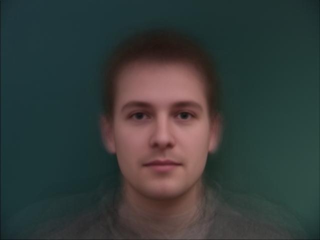
Here is the average face of the population:
Here are some examples of the faces in the dataset being warped into the average shape of the population:
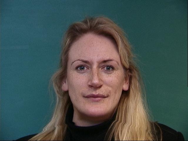
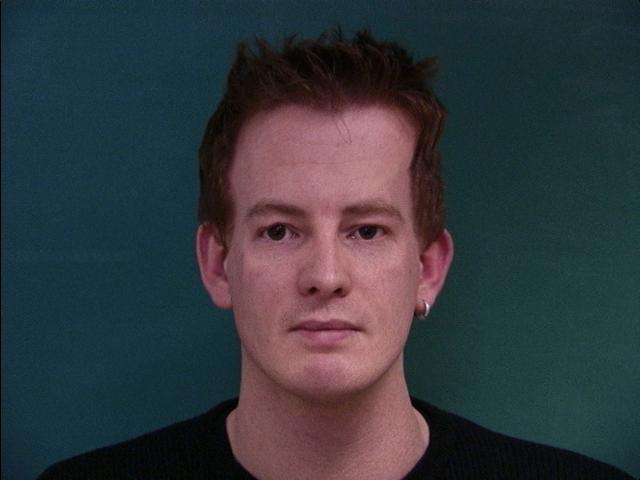
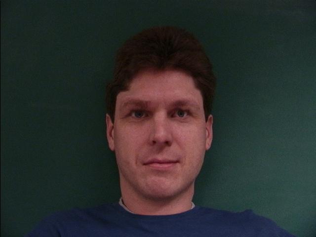
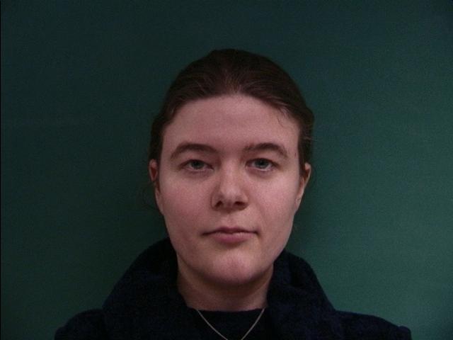
Here is the image of my face warped into the average face of the population:

The main reason for the weird distortions in from my warped face is the misalignment of the original images and the fact that I created the keypoints from my face using a specific image from the Danes dataset rather than using the average shape and average face. As a result, the result in this part and the caricatures in the following parts will also look a little off.
Here is the image of the average face of the population warped into my geometry:
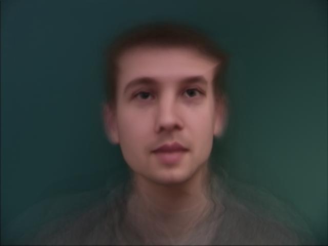
Here, the warped average face is skinnier and the lip is also fuller, which are the two noticeable characteristics of my portrait.
6. Caricatures: Extrapolating from the mean
To extrapolate from the mean, I add the points of my face to a alpha-scaled difference between the points of my face and the points of the mean face. That is, I calculated pts_average = (1 - warp_frac) * im1_pts + warp_frac * im2_pts. I then warped my face into this set of points to obtain the following images:
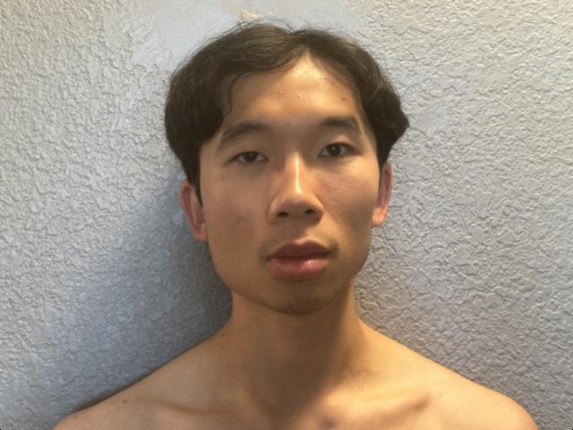
\(\alpha = -0.3\)

\(\alpha = -0.7\)
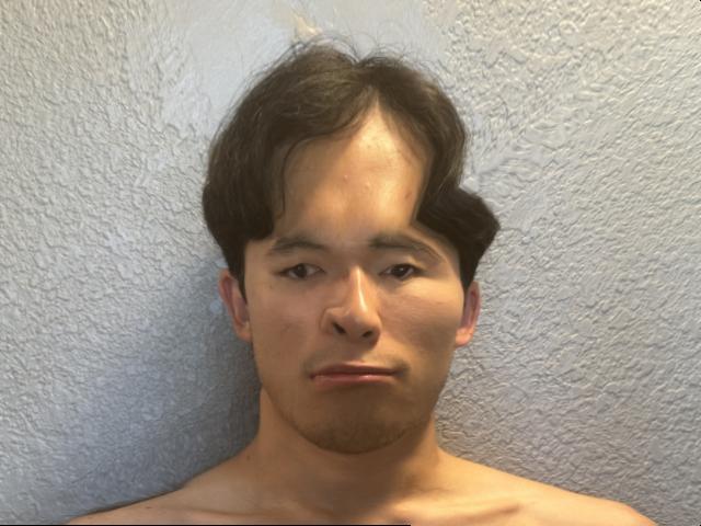
\(\alpha = 1.3\)
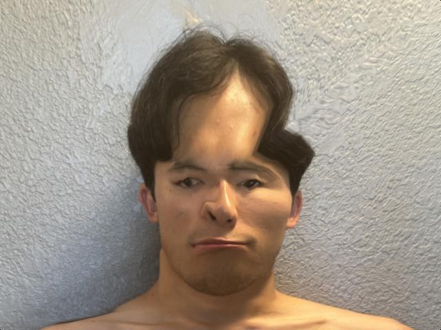
\(\alpha = 1.7\)
According to the project spec, creating caricatures might work better on a gender specific mean. As a result, I repeated the same extrapolation process and instead of using the population's mean, I used the mean of all the male in the Danes population. Here are the images that I obtained:
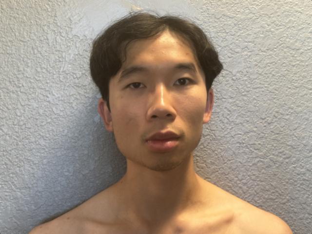
\(\alpha = -0.3\)
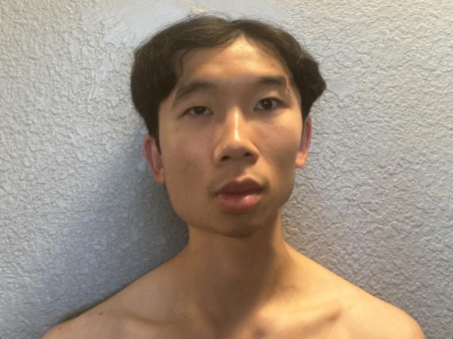
\(\alpha = -0.7\)
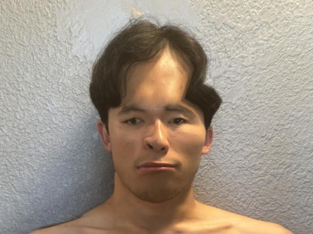
\(\alpha = 1.3\)
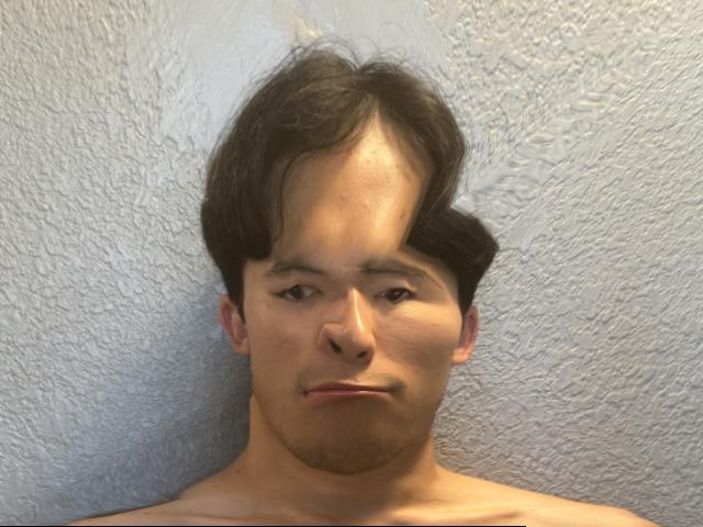
\(\alpha = 1.7\)
The caricatures obtained from the two population look the same for a specific value of \(\alpha\), but if we look closely, the ones obtained from using the average of the male population are little shorter than the corresponding ones from the average of the entire population. This is because the average male face is shorter than the average face of the whole population.
7. Bells and Whistles
7.1. Swapping Gender
I first computed the average face of the female population from the Danes dataset. Here are the three images of just shape warping, just color cross-dissolving, and both:
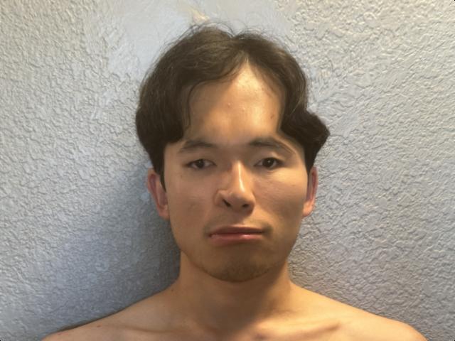
Only shape warping, obtained by warping my face to the geometry of the geometry of the average female face.
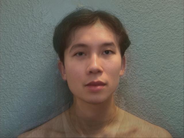
Only cross-dissolving, obtained by warping the average female face to the geometry of my face and then taking the average colors with my face.
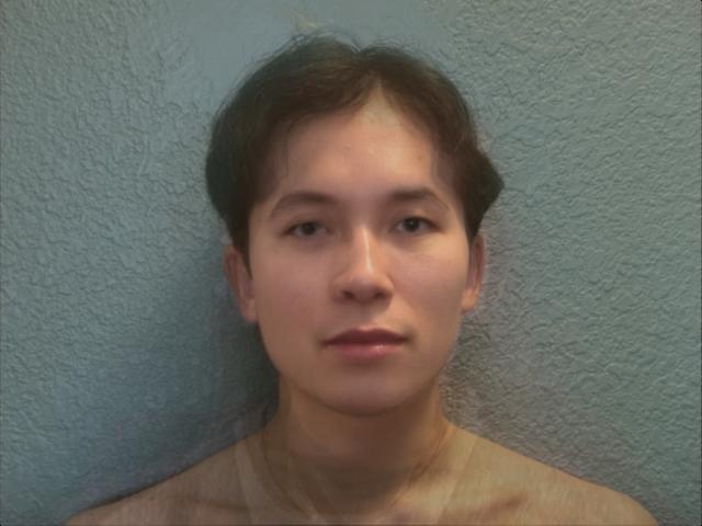
Combining both shape warping and cross-dissolving, using the morph function from Part 3.
As evident from the images, combining both warping and cross-dissolving produces the best and most natural result. Although using cross-dissolving by itself produces a nice color, the resulting shape is not consistent with that of the average female face.
7.2. PCA
I computed the PCA basis for the Danes dataset using sklearn.decomposition.PCA. Here are the first 9 components/eigenfaces of the PCA basis of the Danes dataset:
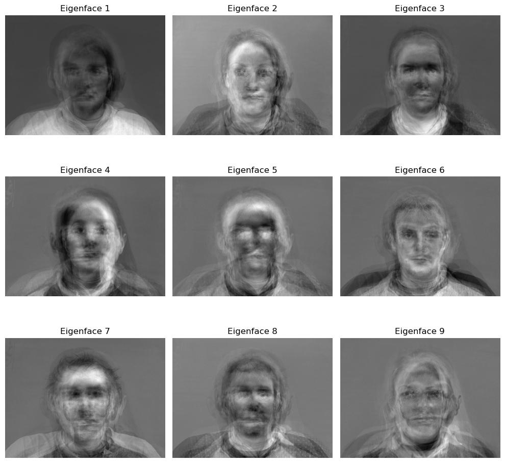
I tried reconstructing the original images using the first k components from the PCA basis:
Reconstruction of Image 0:

Reconstruction of Image 1:

Reconstruction of Image 2:


Notice that for the majority of images, using the first 25 principal components is often sufficient to retrieve a coherent and detailed image. However, for some images, such as Image 2, we need to use more than 25 (35 in the case of Image 2) eigenfaces to have a decent-quality reconstruction.
Here is the mean of the PCA basis that I will use to perform interpolations and extrapolations:
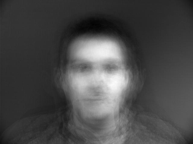
By computing the PCA basis of the set of keypoints, I obtained label_mean, the mean of the PCA basis of all the labels. Using this, I was able to yield the following images:
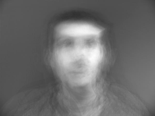
Warping the PCA mean face to my geometry
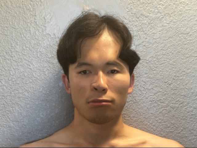
Warping my face to the average geometry of the PCA basis

Caricature with \(\alpha = 1.5\)
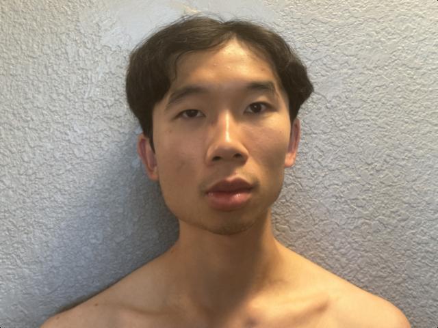
Caricature with \(\alpha = -0.5\)
Aside from the image of warping the PCA mean face to my geometry, which is blurry since the original PCA mean face is also not refined, the remaining images are similar to those computed in the normal basis, primarily because label_mean and the average shape in the normal basis is quite similar.
Here's the image of my face warped and cross-dissolved with the PCA mean face:
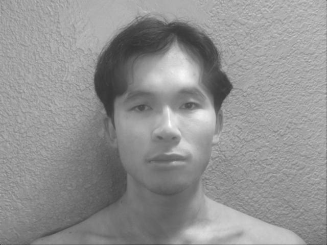
My face warped and cross-dissolved with the PCA mean face

Result of Part 4
In this case, the result from using the PCA basis is much better than the one computed under the normal basis since the left image is less distorted and looks more natural.
I also attemped to perform a gender swap by computing a PCA basis for all the females in the Danes dataset.
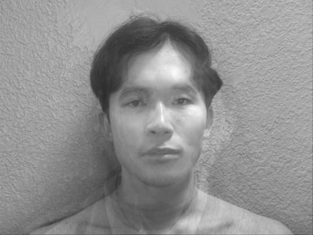
My face warped and cross-dissolved with the PCA mean faceof the female population

Previous Result
For the gender swap, the two images look pretty similar with some minor differences: the face in the right image is a little wider and there's less artifact in the right image. In this situation, using the normal basis yields comparatively better results than using the PCA basis.